Graph Partitioning
If you have a social network where all the people can't fit on one server, a natural question that comes up is how to split up users across machines. There are two main factors to consider:
- For each user, what fraction of their friends stay on the same server.
- Are people evenly distributed between servers.
It's easy to see how these two factors can be in conflict. Trivially all users could be put on just one server, perfectly satisfying the first constraint while soundly failing the second. On the other hand, if we just assigned people randomly to 10 servers, then on average $90\%$ of friendships would span servers. If everyone is friends with everyone else, we can do no better than this $90\%$. However, in most social networks people tend to form little well connected clusters, allowing for far better partitions.
Graph Partitioning
The graph partitioning problem is concerned with breaking up a graph into partitions that maximize edges within each partition while avoid connections that cross groups. Additionally, we would like to optimize balance between the partition sizes.
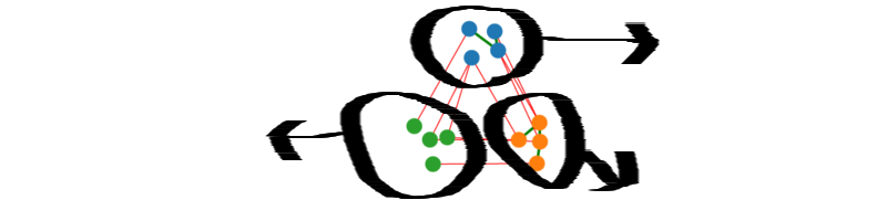
Simple Interactive Example
Below we are trying to break a graph into 3 partitions. The ratio of red edges to total edges is objective 1 to minimize. The other component to minimize is wasted space. We assume that our bin size is just big enough to fit the largest partition, so the "Wasted Bins" metric is the wasted space in the other 2 partitions. For example, if all nodes are in one partition the waste would be 2. If nodes were evenly divided between the 3 partitions, wasted space would be 0. Clicking on a node below will send it to the next partition. Click the nodes below to send them to different partitions and get a sense of the problem.
Real Data
We want to actually evaluate how well we can partition on a real dataset. The Stanford Network Analysis Project is a great place to get realistic social network datasets. We will be working with the Livejournal graph that they have.
You should download the IPython Notebook that goes along with this (or just view it on nbviewer. Provided you have installed Anaconda, it's just a matter of downloading the notebook and running ipython notebook 20131213-graph-partitioning.ipynb. It's definitely more informative to play along and tweak things yourself here.
We will work in numpy. The graph is undirected (after a little pre-processing), and we will just work with a list of edges, since a $[2:\textrm{NUM_EDGES}*2]$ matrix will be convenient and fast. Algorithms will take in a list of edges, and will output an array, $\textrm{NUM_NODES}$ long that has the assignments of nodes to partitions. Our scoring function will thus look like this:
def score(assignment, edges):
    """Compute the score given an assignment of vertices.

    N nodes are assigned to clusters 0 to K-1.

    assignment: Vector where N[i] is the cluster node i is assigned to.
    edges: The edges in the graph, assumed to have one in each direction

    Returns: (total wasted bin space, ratio of edges cut)
    """
    balance = np.bincount(assignment) / len(assignment)
    waste = (np.max(balance) - balance).sum()

    left_edge_assignment = assignment.take(edges[:,0])
    right_edge_assignment = assignment.take(edges[:,1])
    mismatch = (left_edge_assignment != right_edge_assignment).sum()
    cut_ratio = mismatch / len(edges)
    return (waste, cut_ratio)
All algorithms explored will be streaming algorithms. A streaming algorithm is one that does not need to hold the entire dataset in memory, generally making decisions based on local heuristics. Our algorithms will need to hold only a vector of length $\textrm{NUM_NODES}$ in memory. For a graph like Livejournal, there are around 5M nodes, while there are 68M edges. Most other social networks will also have a huge number of edges compared to the number of nodes. In our implementation, we actually do have all the edges in memory too, but it is not a necessity, and would be dropped in a large distributed setting.
Our first approach to partitioning the graph comes from a paper by I. Stanton and G. Kliot. That paper examines many heuristics for the streaming partitioning problem. The best performing one, "Linear Deterministic Greedy", assigns a node a partition based on maximizing the product between how many neighbors a node has in a partition and how full the partition is. For choosing between clusters $1$ through $k$, it picks $i$ as to minimize:
$$ | P_i \cap N(u) | (1 - \frac{P_i}{C_i}) $$
Where $P_i$ is the set of nodes in partition $i$, and $C_i$ is the capacity, which we take to be $\textrm{NUM_NODES} / \textrm{#partitions}$.
Running this algorithm once on the dataset to partition the Livejournal graph into $4$ pieces gives a cut ratio of $.367$ with a waste of $0$. This is much better than random, which would give a cut ratio of $.75$. What's interesting though is if we iterate on the algorithm. The first time the algorithm runs, it likely made some big mistakes in separating a node from its buddies. If however we re-run the algorithm on the dataset, passing in previous assignments, it will allow the algorithm to re-assign nodes to better clusters. This is the idea of a paper by my friends J. Nishimura and J. Ugander where they call this operation "restreaming". Taking the simple LDG algorithm, and modifying slightly for restreaming, we arrive at the following algorithm:
%%cython
import numpy as np
cimport cython

cdef int UNMAPPED = -1

def linear_deterministic_greedy(int[:,::] edges,
                                int num_nodes,
                                int num_partitions,
                                int[::] partition):
    """
    This algorithm favors a cluster if it has many neighbors of a node, but
    penalizes the cluster if it is close to capacity.

    edges: An [:,2] array of edges.
    num_nodes: The number of nodes in the graph.
    num_partitions: How many partitions we are breaking the graph into.
    partition: The partition from a previous run. Used for restreaming.

    Returns: A new partition.
    """
    # The output partition

    if partition is None:
        partition = np.repeat(np.int32(UNMAPPED), num_nodes)

    cdef int[::] partition_sizes = np.zeros(num_partitions, dtype=np.int32)

    cdef int[::] partition_votes = np.zeros(num_partitions, dtype=np.int32)

    # Fine to be a little off, to stay integers
    cdef int partition_capacity = num_nodes / num_partitions

    cdef int last_left = edges[0,0]
    cdef int i = 0
    cdef int left = 0
    cdef int right = 0
    cdef int arg = 0
    cdef int max_arg = 0
    cdef int max_val = 0
    cdef int val = 0
    cdef int len_edges = len(edges)

    for i in range(len_edges):
        left = edges[i,0]
        right = edges[i,1]

        if last_left != left:
            # We have found a new node so assign last_left to a partition

            max_arg = 0
            max_val = (partition_votes[0]) * (
                       partition_capacity - partition_sizes[0])

            for arg in range(1, num_partitions):
                val = (partition_votes[arg]) * (
                       partition_capacity - partition_sizes[arg])
                if val > max_val:
                    max_arg = arg
                    max_val = val

            if max_val == 0:
                max_arg = arg
                # No neighbors (or multiple maxed out) so "randomly" select
                # the smallest partition
                for arg in range(i % num_partitions, num_partitions):
                    if partition_sizes[arg] < partition_capacity:
                        max_arg = arg
                        max_val = 1
                        break
                if max_val == 0:
                    for arg in range(0, i % num_partitions):
                        if partition_sizes[arg] < partition_capacity:
                            max_arg = arg
                            break


            partition_sizes[max_arg] += 1
            partition[last_left] = max_arg
            partition_votes[:] = 0
            last_left = left

        if partition[right] != UNMAPPED:
            partition_votes[partition[right]] += 1


    # Clean up the last assignment
    max_arg = 0
    max_val = 0
    for arg in range(0, num_partitions):
        if partition_sizes[arg] < partition_capacity:
            val = (partition_votes[arg]) * (
                    1 - partition_sizes[arg] / partition_capacity)
            if val > max_val:
                max_arg = arg
                max_val = val
    partition[left] = max_arg

    return np.asarray(partition)
I posted that in part to show off Cython. All that's really going is that we pass the old partitions in to the algorithm on its next run, and it uses those values in the $| P_i \cap N(u) |$ calculation. We rank partitions taking into account how full it is this round, and how many of of neighbors have been assigned there this round or last round. Using this approach, we we can quickly converge to a much better solution!
# Use the greedy method to break into 4 partitions
%time run_restreaming_greedy(edges, NUM_NODES, num_partitions=4, num_iterations=15)

Fennel
It's nice to see how well that simple rule works to give a fairly decent partition. In our next Graph Partitioning post, we'll examine an algorithm called FENNEL which we can push to even better partitions. Download the IPython Notebook to see an implementation. Here's an initial teaser though!
%time run_fennel_restreaming(edges, NUM_NODES, 4, 15)

Next Steps
Running LDG on the unshuffled edges in the attached IPython notebook actually performs better than LDG and FENNEL in the J. Nishimura and J. Ugander paper. The original ordering of the nodes had some properties that made it far better than a random ordering. In the notebook I have shuffled and unshuffled input. It will be informative to try to figure out what exactly the difference is in the local topology of the early nodes. Running LDG on the unshuffled edges gives better performance than running FENNEL on the shuffled edges. There are definitely some interesting rules to discover for optimal node ordering in this problem. Johan Ugunder remarked that the original ordering likely reflected a certain traversal ordering of the Livejournal graph, and that traversal ordering has some deep ramifications in related problems like web graph compression.
Thanks!
A huge thanks to Joel Nishimura for tons of help in replicating his results, and in giving future research directions. I would also like to thank Johans Ugander for looking over this post and giving some insight as to why random ordering impacted performance.